 |
| BS1.5: Probability Distributions |
 |
| BS1.5: Probability Distributions |
OBJECTIVES |
At the end of this section you should be able to:
|
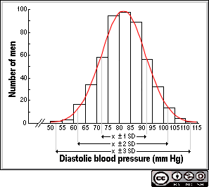
Numerical variables, such as the distribution body weights, heights, blood pressure measurements in the general population tend to approximately follow a bell-shaped curve, commonly referred to as the Normal distribution or Gaussian distribution. This distribution is symmetrical about its mean.
For a normal distribution", a range covered by:
mean ± 1 SD includes about 68% of the observations
mean ± 2 SD includes about 95% of the observations
mean ± 3 SD includes about 99% of the observations.

The figure above show a normal distribution of diastolic blood pressure measurements among 500 men with mean=82 mm Hg and standard deviation=10 mm Hg.
The probability limits within two standard deviations of the mean is:
mean ± 2 SD
82 ± 2 (10)
62 ; 102
Approximately 95% of the diastolic blood pressure measurements lies between 62 and 102 mm Hg.
A proportion (p) is calculated from a binary variable, where each individual in the sample is assigned to one of two alternatives.
Proportion: p = r / n
where r = number of individuals with the characteristics and n = sample size.
The sampling distribution for the proportion is called the Binomial distribution.
The proportion of smokers among a sample of female clothing factory workers:
r = 60 smokers
n = 300 female workers
gives the proportion, p = 60/300 = 0.20.
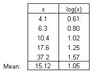
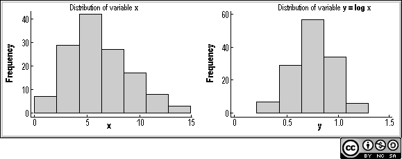
Variables that are not normally distributed can be made so by a suitable transformation. When a distribution is skewed the assumptions underlying a statistical method may not be satisfied, and this can be overcome by transforming the data to a different scale of measurement. The most commonly used transformation is the logarithm. When we applying a logarithmic transformation each individual value is replaced by its logarithm
y = log x
Where x is the original value and y the transformed value.
| The antilog of 1.05 is 11.2, called the Geometric mean. |  |

