RESULTS:

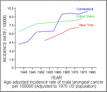
Investigators decided to use all three sets of comparison rates and calculate a range of results. Figure 3.1 shows the rates that were available. Lines have been drawn between the points, but actual rates were available only at the calendar times indicated by the points. Figure 3.1 shows that Connecticut rates were highest for the period from 1960 on, while New York rates were lowest. Given that the points in the figure shown below for the respective locations appear to increase more or less linearly over time, investigators used simple linear regression to determine a best-fitting line for rates over time. For example, rates for 1949 to 1969 in the United States were determined using this regression procedure, since existing data were limited to 1948 and 1970 (in actuality, separate regressions were run for each set of age-specific rates).

The next problem was the method of control over smoking and drinking. Smoking and drinking habits of the cohort were known from the questionnaires, and smoking- and drinking-specific laryngeal cancer rates could be calculated. However, analogous smoking and drinking-specific laryngeal cancer rates were not available for any of the comparison populations. If they had been available, they would have allowed good control over confounding via stratification (the same technique used for age and calendar time). Exposed smokers would have been compared to nonexposed smokers, exposed nonsmokers to nonexposed nonsmokers, etc., and then a weighted average of these rate ratios would have been calculated.

Lacking such data, however, investigators needed other methods. There were some data on the smoking and drinking habits of the V.S. population at various times. Investigators decided to use an adjustment, known as the Axelson adjustment, to try to determine the effects of differing smoking and drinking habits between the exposed and nonexposed (Axelson, 1978). Inspection of the smoking and drinking habits of the exposed versus the nonexposed allowed the investigators to determine if they differed. If they did not differ, then smoking and drinking would not act as confounders and would not need to be controlled in the analysis. Suppose, however, they did differ. Suppose the exposed population smoked and drank more, for example, than did the comparison population. The Axelson technique would use the known effects of smoking and drinking on larynx cancer rates to predict how much difference in larynx cancer rates between exposed and nonexposed would be expected to occur due to smoking and drinking, under the assumption that there was no effect of exposure to acid mists whatsoever. Any difference in larynx cancer rates above and beyond those predicted by excess smoking and drinking by the exposed cohort might then be attributed to exposure to acid mists.

The Table below shows the questionnaire response rates for the study population. As expected, response rates for next of kin were worse than response rates for those still alive. The bulk of the nonresponse for the next of kin was due to the inability of the investigators to locate the next of kin, rather than refusal to complete the questionnaire.

QUESTIONS

After considering the above, try and answer the following questions:

1. QUESTION 4. Why is it important that comparison rates be age-specific and specific to particular calendar periods?
2. QUESTION 5. What problems would you anticipate in using these rates as nonexposed comparison rates for this study? Which would you use?
3. QUESTION 6. In what ways could the level of nonresponse cause the study results to be invalid?